Knowledge Base Wiki

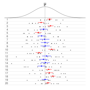
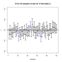
Informally, in frequentist statistics, a confidence interval (CI) is an interval which is expected to typically contain the parameter being estimated. More specifically, given a confidence level $\gamma$ (95% and 99% are typical values), a CI is a random interval which contains the parameter being estimated $\gamma$ % of the time.^[1]^[2] The confidence level, degree of confidence or confidence coefficient represents the long-run proportion of CIs (at the given confidence level) that theoretically contain the true value of the parameter; this is tantamount to the nominal coverage probability. For example, out of all intervals computed at the 95% level, 95% of them should contain the parameter's true value.^[3]

Factors affecting the width of the CI include the sample size, the variability in the sample, and the confidence level.^[4] All else being the same, a larger sample produces a narrower confidence interval, greater variability in the sample produces a wider confidence interval, and a higher confidence level produces a wider confidence interval.^[5]

History

Methods for calculating confidence intervals for the binomial proportion appeared from the 1920s.^[6]^[7] The main ideas of confidence intervals in general were developed in the early 1930s,^[8]^[9]^[10] and the first thorough and general account was given by Jerzy Neyman in 1937.^[11]

Neyman described the development of the ideas as follows (reference numbers have been changed):^[10]

[My work on confidence intervals] originated about 1930 from a simple question of Waclaw Pytkowski, then my student in Warsaw, engaged in an empirical study in farm economics. The question was: how to characterize non-dogmatically the precision of an estimated regression coefficient? ...
Pytkowski's monograph ... appeared in print in 1932.^[12] It so happened that, somewhat earlier, Fisher published his first paper^[13] concerned with fiducial distributions and fiducial argument. Quite unexpectedly, while the conceptual framework of fiducial argument is entirely different from that of confidence intervals, the specific solutions of several particular problems coincided. Thus, in the first paper in which I presented the theory of confidence intervals, published in 1934,^[8] I recognized Fisher's priority for the idea that interval estimation is possible without any reference to Bayes' theorem and with the solution being independent from probabilities a priori. At the same time I mildly suggested that Fisher's approach to the problem involved a minor misunderstanding.

In medical journals, confidence intervals were promoted in the 1970s but only became widely used in the 1980s.^[14] By 1988, medical journals were requiring the reporting of confidence intervals.^[15]

Definition

Let $X$ be a random sample from a probability distribution with statistical parameter $\theta$ , which is a quantity to be estimated, and $\varphi$ , representing quantities that are not of immediate interest. A confidence interval for the parameter $\theta$ , with confidence level or coefficient $\gamma$ , is an interval $(u(X),v(X))$ determined by random variables $u(X)$ and $v(X)$ with the property:

P(u(X)<\theta <v(X))=\gamma \quad {\text{ for every }}(\theta ,\varphi ).

The number $\gamma$ , whose typical value is close to but not greater than 1, is sometimes given in the form $1-\alpha$ (or as a percentage $100\%\cdot (1-\alpha )$ ), where $\alpha$ is a small positive number, often 0.05.

It is important for the bounds $u(X)$ and $v(X)$ to be specified in such a way that as long as $X$ is collected randomly, every time we compute a confidence interval, there is probability $\gamma$ that it would contain $\theta$ , the true value of the parameter being estimated. This should hold true for any actual $\theta$ and $\varphi$ .^[2]

Approximate confidence intervals

In many applications, confidence intervals that have exactly the required confidence level are hard to construct, but approximate intervals can be computed. The rule for constructing the interval may be accepted as providing a confidence interval at level $\gamma$ if

P(u(X)<\theta <v(X))\approx \ \gamma \quad {\text{ for every }}(\theta ,\varphi )

to an acceptable level of approximation. Alternatively, some authors^[16] simply require that

P(u(X)<\theta <v(X))\geq \ \gamma \quad {\text{ for every }}(\theta ,\varphi ),

which is useful if the probabilities are only partially identified or imprecise, and also when dealing with discrete distributions. Confidence limits of the form

P(u(X)<\theta )\geq \ \gamma

and

P(\theta <v(X))\geq \gamma

are called conservative;^[17]^(p 210) accordingly, one speaks of conservative confidence intervals and, in general, regions.

Desired properties

When applying standard statistical procedures, there will often be standard ways of constructing confidence intervals. These will have been devised so as to meet certain desirable properties, which will hold given that the assumptions on which the procedure relies are true. These desirable properties may be described as: validity, optimality, and invariance.

Of the three, "validity" is most important, followed closely by "optimality". "Invariance" may be considered as a property of the method of derivation of a confidence interval, rather than of the rule for constructing the interval. In non-standard applications, these same desirable properties would be sought:

Validity

This means that the nominal coverage probability (confidence level) of the confidence interval should hold, either exactly or to a good approximation.

Optimality

This means that the rule for constructing the confidence interval should make as much use of the information in the data-set as possible.

One way of assessing optimality is by the width of the interval so that a rule for constructing a confidence interval is judged better than another if it leads to intervals whose widths are typically shorter.

Invariance

In many applications, the quantity being estimated might not be tightly defined as such.

For example, a survey might result in an estimate of the median income in a population, but it might equally be considered as providing an estimate of the logarithm of the median income, given that this is a common scale for presenting graphical results. It would be desirable that the method used for constructing a confidence interval for the median income would give equivalent results when applied to constructing a confidence interval for the logarithm of the median income: Specifically the values at the ends of the latter interval would be the logarithms of the values at the ends of former interval.

Methods of derivation

For non-standard applications, there are several routes that might be taken to derive a rule for the construction of confidence intervals. Established rules for standard procedures might be justified or explained via several of these routes. Typically a rule for constructing confidence intervals is closely tied to a particular way of finding a point estimate of the quantity being considered.

Summary statistics

This is closely related to the method of moments for estimation. A simple example arises where the quantity to be estimated is the population mean, in which case a natural estimate is the sample mean. Similarly, the sample variance can be used to estimate the population variance. A confidence interval for the true mean can be constructed centered on the sample mean with a width which is a multiple of the square root of the sample variance.

Likelihood theory

Estimates can be constructed using the maximum likelihood principle, the likelihood theory for this provides two ways of constructing confidence intervals or confidence regions for the estimates.

Estimating equations

The estimation approach here can be considered as both a generalization of the method of moments and a generalization of the maximum likelihood approach. There are corresponding generalizations of the results of maximum likelihood theory that allow confidence intervals to be constructed based on estimates derived from estimating equations.^{[citation needed]}

Hypothesis testing

If hypothesis tests are available for general values of a parameter, then confidence intervals/regions can be constructed by including in the 100 $p$ % confidence region all those points for which the hypothesis test of the null hypothesis that the true value is the given value is not rejected at a significance level of (1 − $p$ ).^[17]^{(§ 7.2 (iii))}

Bootstrapping

In situations where the distributional assumptions for the above methods are uncertain or violated, resampling methods allow construction of confidence intervals or prediction intervals. The observed data distribution and the internal correlations are used as the surrogate for the correlations in the wider population.

Central limit theorem

The central limit theorem is a refinement of the law of large numbers. For a large number of independent identically distributed random variables $X_{1},...,X_{n},$ with finite variance, the average ${\overline {X}}_{n}$ approximately has a normal distribution, no matter what the distribution of the $X_{i}$ is, with the approximation roughly improving in proportion to ${\sqrt {n}}$ .^[2]

Example

In this bar chart, the top ends of the brown bars indicate observed means and the red line segments ("error bars") represent the confidence intervals around them. Although the error bars are shown as symmetric around the means, that is not always the case. In most graphs, the error bars do not represent confidence intervals (e.g., they often represent standard errors or standard deviations).

Suppose ${X_{1},\ldots ,X_{n}}$ is an independent sample from a normally distributed population with unknown parameters mean $\mu$ and variance $\sigma ^{2}.$ Let

{\bar {X}}={\frac {X_{1}+\cdots +X_{n}}{n}},

S^{2}={\frac {1}{n-1}}\sum _{i=1}^{n}(X_{i}-{\bar {X}})^{2}.

Where ${\bar {X}}$ is the sample mean, and $S^{2}$ is the sample variance. Then

T={\frac {{\bar {X}}-\mu }{S/{\sqrt {n}}}}

has a Student's t distribution with $n-1$ degrees of freedom.^[18] Note that the distribution of $T$ does not depend on the values of the unobservable parameters $\mu$ and $\sigma ^{2}$ ; i.e., it is a pivotal quantity. Suppose we wanted to calculate a 95% confidence interval for $\mu .$ Then, denoting $c$ as the 97.5th percentile of this distribution,

P_{T}(-c\leq T\leq c)=0.95.

Note that "97.5th" and "0.95" are correct in the preceding expressions. There is a 2.5% chance that $T$ will be less than $-c$ and a 2.5% chance that it will be larger than $+c.$ Thus, the probability that $T$ will be between $-c$ and $+c$ is 95%. $P_{T}$ is the probability measure under the student $t$ distribution.

Consequently,

P_{\mu }\left({\bar {X}}-{\frac {cS}{\sqrt {n}}}\leq \mu \leq {\bar {X}}+{\frac {cS}{\sqrt {n}}}\right)=0.95,

and we have a theoretical (stochastic) 95% confidence interval for $\mu .$ Here $P_{\mu }$ is the probability measure under unknown distribution of $\mu$ .

After observing the sample we find values ${\bar {x}}$ for ${\bar {X}}$ and $s$ for $S,$ from which we compute the confidence interval

\left[{\bar {x}}-{\frac {cs}{\sqrt {n}}},{\bar {x}}+{\frac {cs}{\sqrt {n}}}\right].

Interpretation

Various interpretations of a confidence interval can be given (taking the 95% confidence interval as an example in the following).

The confidence interval can be expressed in terms of a long-run frequency in repeated samples (or in resampling): "Were this procedure to be repeated on numerous samples, the proportion of calculated 95% confidence intervals that encompassed the true value of the population parameter would tend toward 95%."^[19]
The confidence interval can be expressed in terms of probability with respect to a single theoretical (yet to be realized) sample: "There is a 95% probability that the 95% confidence interval calculated from a given future sample will cover the true value of the population parameter."[11] This essentially reframes the "repeated samples" interpretation as a probability rather than a frequency.
The confidence interval can be expressed in terms of statistical significance, e.g.: "The 95% confidence interval represents values that are not statistically significantly different from the point estimate at the .05 level."^[20]

Common misunderstandings

Confidence intervals and levels are frequently misunderstood, and published studies have shown that even professional scientists often misinterpret them.^[21]^[22]^[23]^[24]^[25]^[26]

A 95% confidence level does not mean that for a given realized interval there is a 95% probability that the population parameter lies within the interval (i.e., a 95% probability that the interval covers the population parameter).^[27] According to the frequentist interpretation, once an interval is calculated, this interval either covers the parameter value or it does not; it is no longer a matter of probability. The 95% probability relates to the reliability of the estimation procedure, not to a specific calculated interval.^[28] Neyman himself (the original proponent of confidence intervals) made this point in his original paper:^[11]
It will be noticed that in the above description, the probability statements refer to the problems of estimation with which the statistician will be concerned in the future. In fact, I have repeatedly stated that the frequency of correct results will tend to α. Consider now the case when a sample is already drawn, and the calculations have given [particular limits]. Can we say that in this particular case the probability of the true value [falling between these limits] is equal to α? The answer is obviously in the negative. The parameter is an unknown constant, and no probability statement concerning its value may be made...

A 95% confidence level does not mean that 95% of the sample data lie within the confidence interval.
A 95% confidence level does not mean that there is a 95% probability of the parameter estimate from a repeat of the experiment falling within the confidence interval computed from a given experiment.^[25]

Examples of how naïve interpretation of confidence intervals can be problematic

Confidence procedure for uniform location

Welch^[29] presented an example which clearly shows the difference between the theory of confidence intervals and other theories of interval estimation (including Fisher's fiducial intervals and objective Bayesian intervals). Robinson^[30] called this example "[p]ossibly the best known counterexample for Neyman's version of confidence interval theory." To Welch, it showed the superiority of confidence interval theory; to critics of the theory, it shows a deficiency. Here we present a simplified version.

Suppose that $X_{1},X_{2}$ are independent observations from a uniform $(\theta -1/2,\theta +1/2)$ distribution. Then the optimal 50% confidence procedure for $\theta$ is^[31]

{\bar {X}}\pm {\begin{cases}{\dfrac {|X_{1}-X_{2}|}{2}}&{\text{if }}|X_{1}-X_{2}|<1/2\\[8pt]{\dfrac {1-|X_{1}-X_{2}|}{2}}&{\text{if }}|X_{1}-X_{2}|\geq 1/2.\end{cases}}

A fiducial or objective Bayesian argument can be used to derive the interval estimate

{\bar {X}}\pm {\frac {1-|X_{1}-X_{2}|}{4}},

which is also a 50% confidence procedure. Welch showed that the first confidence procedure dominates the second, according to desiderata from confidence interval theory; for every $\theta _{1}\neq \theta$ , the probability that the first procedure contains $\theta _{1}$ is less than or equal to the probability that the second procedure contains $\theta _{1}$ . The average width of the intervals from the first procedure is less than that of the second. Hence, the first procedure is preferred under classical confidence interval theory.

However, when $|X_{1}-X_{2}|\geq 1/2$ , intervals from the first procedure are guaranteed to contain the true value $\theta$ : Therefore, the nominal 50% confidence coefficient is unrelated to the uncertainty we should have that a specific interval contains the true value. The second procedure does not have this property.

Moreover, when the first procedure generates a very short interval, this indicates that $X_{1},X_{2}$ are very close together and hence only offer the information in a single data point. Yet the first interval will exclude almost all reasonable values of the parameter due to its short width. The second procedure does not have this property.

The two counter-intuitive properties of the first procedure – 100% coverage when $X_{1},X_{2}$ are far apart and almost 0% coverage when $X_{1},X_{2}$ are close together – balance out to yield 50% coverage on average. However, despite the first procedure being optimal, its intervals offer neither an assessment of the precision of the estimate nor an assessment of the uncertainty one should have that the interval contains the true value.

This example is used to argue against naïve interpretations of confidence intervals. If a confidence procedure is asserted to have properties beyond that of the nominal coverage (such as relation to precision, or a relationship with Bayesian inference), those properties must be proved; they do not follow from the fact that a procedure is a confidence procedure.

Confidence procedure for ω²

Steiger^[32] suggested a number of confidence procedures for common effect size measures in ANOVA. Morey et al.^[27] point out that several of these confidence procedures, including the one for ω², have the property that as the F statistic becomes increasingly small—indicating misfit with all possible values of ω²—the confidence interval shrinks and can even contain only the single value ω² = 0; that is, the CI is infinitesimally narrow (this occurs when $p\geq 1-\alpha /2$ for a $100(1-\alpha )\%$ CI).

This behavior is consistent with the relationship between the confidence procedure and significance testing: as F becomes so small that the group means are much closer together than we would expect by chance, a significance test might indicate rejection for most or all values of ω². Hence the interval will be very narrow or even empty (or, by a convention suggested by Steiger, containing only 0). However, this does not indicate that the estimate of ω² is very precise. In a sense, it indicates the opposite: that the trustworthiness of the results themselves may be in doubt. This is contrary to the common interpretation of confidence intervals that they reveal the precision of the estimate.

References

^ Zar, Jerrold H. (199). Biostatistical Analysis (4th ed.). Upper Saddle River, N.J.: Prentice Hall. pp. 43–45. ISBN 978-0130815422. OCLC 39498633.
^ ^a ^b ^c Dekking, Frederik Michel; Kraaikamp, Cornelis; Lopuhaä, Hendrik Paul; Meester, Ludolf Erwin (2005). "A Modern Introduction to Probability and Statistics". Springer Texts in Statistics. doi:10.1007/1-84628-168-7. ISBN 978-1-85233-896-1. ISSN 1431-875X.
^ Illowsky, Barbara. Introductory statistics. Dean, Susan L., 1945-, Illowsky, Barbara., OpenStax College. Houston, Texas. ISBN 978-1-947172-05-0. OCLC 899241574.
^ Hazra, Avijit (October 2017). "Using the confidence interval confidently". Journal of Thoracic Disease. 9 (10): 4125–4130. doi:10.21037/jtd.2017.09.14. ISSN 2072-1439. PMC 5723800. PMID 29268424.
^ Khare, Vikas; Nema, Savita; Baredar, Prashant (2020). Ocean Energy Modeling and Simulation with Big Data Computational Intelligence for System Optimization and Grid Integration. Butterworth-Heinemann. ISBN 978-0-12-818905-4. OCLC 1153294021.
^ Edwin B. Wilson (1927) Probable Inference, the Law of Succession, and Statistical Inference, Journal of the American Statistical Association, 22:158, 209-212, https://doi.org/10.1080/01621459.1927.10502953
^ C.J. Clopper, E.S. Pearson, The use of confidence or fiducial limits illustrated in the case of the binomial, Biometrika 26(4), 1934, pages 404–413, https://doi.org/10.1093/biomet/26.4.404
^ ^a ^b Neyman, J. (1934). On the Two Different Aspects of the Representative Method: The Method of Stratified Sampling and the Method of Purposive Selection. Journal of the Royal Statistical Society, 97(4), 558–625. https://doi.org/10.2307/2342192 (see Note I in the appendix)
^ J. Neyman (1935), Ann. Math. Statist. 6(3): 111-116 (September, 1935). https://doi.org/10.1214/aoms/1177732585
^ ^a ^b Neyman, J. (1970). A glance at some of my personal experiences in the process of research. In Scientists at Work: Festschrift in honour of Herman Wold. Edited by T. Dalenius, G. Karlsson, S. Malmquist. Almqvist & Wiksell, Stockholm. https://worldcat.org/en/title/195948
^ ^a ^b ^c Neyman, J. (1937). "Outline of a Theory of Statistical Estimation Based on the Classical Theory of Probability". Philosophical Transactions of the Royal Society A. 236 (767): 333–380. Bibcode:1937RSPTA.236..333N. doi:10.1098/rsta.1937.0005. JSTOR 91337.
^ Pytkowski, W., The dependence of the income in small farms upon their area, the outlay and the capital invested in cows. (Polish, English summary) Bibliotaka Palawska, 1932.
^ Fisher, R. (1930). Inverse Probability. Mathematical Proceedings of the Cambridge Philosophical Society, 26(4), 528-535. https://doi.org/10.1017/S0305004100016297
^ Altman, Douglas G. (1991). "Statistics in medical journals: Developments in the 1980s". Statistics in Medicine. 10 (12): 1897–1913. doi:10.1002/sim.4780101206. ISSN 1097-0258. PMID 1805317.
^ Gardner, Martin J.; Altman, Douglas G. (1988). "Estimating with confidence". British Medical Journal. 296 (6631): 1210–1211. doi:10.1136/bmj.296.6631.1210. PMC 2545695. PMID 3133015.
^ Roussas, George G. (1997). A Course in Mathematical Statistics (2nd ed.). Academic Press. p. 397.
^ ^a ^b Cox, D.R.; Hinkley, D.V. (1974). Theoretical Statistics. Chapman & Hall.
^ Rees, D.G. (2001). Essential Statistics, 4th Edition, Chapman and Hall/CRC. ISBN 1-58488-007-4 (Section 9.5)
^ Cox D.R., Hinkley D.V. (1974) Theoretical Statistics, Chapman & Hall, p49, p209
^ Cox D.R., Hinkley D.V. (1974) Theoretical Statistics, Chapman & Hall, pp. 214, 225, 233
^ Kalinowski, Pawel (2010). "Identifying Misconceptions about Confidence Intervals" (PDF). Retrieved 2021-12-22.
^ "Archived copy" (PDF). Archived from the original (PDF) on 2016-03-04. Retrieved 2014-09-16.{{cite web}}: CS1 maint: archived copy as title (link)
^ Hoekstra, R., R. D. Morey, J. N. Rouder, and E-J. Wagenmakers, 2014. Robust misinterpretation of confidence intervals. Psychonomic Bulletin & Review Vol. 21, No. 5, pp. 1157-1164. [1]
^ Scientists' grasp of confidence intervals doesn't inspire confidence, Science News, July 3, 2014
^ ^a ^b Greenland, Sander; Senn, Stephen J.; Rothman, Kenneth J.; Carlin, John B.; Poole, Charles; Goodman, Steven N.; Altman, Douglas G. (April 2016). "Statistical tests, P values, confidence intervals, and power: a guide to misinterpretations". European Journal of Epidemiology. 31 (4): 337–350. doi:10.1007/s10654-016-0149-3. ISSN 0393-2990. PMC 4877414. PMID 27209009.
^ Helske, Jouni; Helske, Satu; Cooper, Matthew; Ynnerman, Anders; Besancon, Lonni (2021-08-01). "Can Visualization Alleviate Dichotomous Thinking? Effects of Visual Representations on the Cliff Effect". IEEE Transactions on Visualization and Computer Graphics. 27 (8). Institute of Electrical and Electronics Engineers (IEEE): 3397–3409. arXiv:2002.07671. doi:10.1109/tvcg.2021.3073466. ISSN 1077-2626. PMID 33856998. S2CID 233230810.
^ ^a ^b Morey, R. D.; Hoekstra, R.; Rouder, J. N.; Lee, M. D.; Wagenmakers, E.-J. (2016). "The Fallacy of Placing Confidence in Confidence Intervals". Psychonomic Bulletin & Review. 23 (1): 103–123. doi:10.3758/s13423-015-0947-8. PMC 4742505. PMID 26450628.
^ "1.3.5.2. Confidence Limits for the Mean". nist.gov. Archived from the original on 2008-02-05. Retrieved 2014-09-16.
^ Welch, B. L. (1939). "On Confidence Limits and Sufficiency, with Particular Reference to Parameters of Location". The Annals of Mathematical Statistics. 10 (1): 58–69. doi:10.1214/aoms/1177732246. JSTOR 2235987.
^ Robinson, G. K. (1975). "Some Counterexamples to the Theory of Confidence Intervals". Biometrika. 62 (1): 155–161. doi:10.2307/2334498. JSTOR 2334498.
^ Pratt, J. W. (1961). "Book Review: Testing Statistical Hypotheses. by E. L. Lehmann". Journal of the American Statistical Association. 56 (293): 163–167. doi:10.1080/01621459.1961.10482103. JSTOR 2282344.
^ Steiger, J. H. (2004). "Beyond the F test: Effect size confidence intervals and tests of close fit in the analysis of variance and contrast analysis". Psychological Methods. 9 (2): 164–182. doi:10.1037/1082-989x.9.2.164. PMID 15137887.

Bibliography

"Confidence estimation", Encyclopedia of Mathematics, EMS Press, 2001 [1994]
Fisher, R.A. (1956) Statistical Methods and Scientific Inference. Oliver and Boyd, Edinburgh. (See p. 32.)
Freund, J.E. (1962) Mathematical Statistics Prentice Hall, Englewood Cliffs, NJ. (See pp. 227–228.)
Hacking, I. (1965) Logic of Statistical Inference. Cambridge University Press, Cambridge. ISBN 0-521-05165-7
Keeping, E.S. (1962) Introduction to Statistical Inference. D. Van Nostrand, Princeton, NJ.
Kiefer, J. (1977). "Conditional Confidence Statements and Confidence Estimators (with discussion)". Journal of the American Statistical Association. 72 (360a): 789–827. doi:10.1080/01621459.1977.10479956. JSTOR 2286460.
Mayo, D. G. (1981) "In defence of the Neyman–Pearson theory of confidence intervals", Philosophy of Science, 48 (2), 269–280. JSTOR 187185.
Mehta, S. (2014) Statistics Topics. ISBN 978-1-4992-7353-3.
Morey, R. D.; Hoekstra, R.; Rouder, J. N.; Lee, M. D.; Wagenmakers, E.-J. (2016). "The fallacy of placing confidence in confidence intervals". Psychonomic Bulletin & Review. 23 (1): 103–123. doi:10.3758/s13423-015-0947-8. PMC 4742505. PMID 26450628.
Neyman, J. (1937) "Outline of a Theory of Statistical Estimation Based on the Classical Theory of Probability" Philosophical Transactions of the Royal Society of London A, 236, 333–380. (Seminal work)
Robinson, G.K. (1975). "Some Counterexamples to the Theory of Confidence Intervals". Biometrika. 62 (1): 155–161. doi:10.1093/biomet/62.1.155. JSTOR 2334498.
Savage, L. J. (1962), The Foundations of Statistical Inference. Methuen, London.
Smithson, M. (2003) Confidence intervals. Quantitative Applications in the Social Sciences Series, No. 140. Belmont, CA: SAGE Publications. ISBN 978-0-7619-2499-9.

External links

The Exploratory Software for Confidence Intervals tutorial programs that run under Excel
Confidence interval calculators for R-Squares, Regression Coefficients, and Regression Intercepts
Weisstein, Eric W. "Confidence Interval". MathWorld.
CAUSEweb.org Many resources for teaching statistics including Confidence Intervals.
An interactive introduction to Confidence Intervals
Confidence Intervals: Confidence Level, Sample Size, and Margin of Error by Eric Schulz, the Wolfram Demonstrations Project.
Confidence Intervals in Public Health Archived 2016-08-09 at the Wayback Machine. Straightforward description with examples and what to do about small sample sizes or rates near 0.

[1] Zar, Jerrold H. (199). Biostatistical Analysis (4th ed.). Upper Saddle River, N.J.: Prentice Hall. pp. 43–45. ISBN 978-0130815422. OCLC 39498633.

[Dekking-2] Dekking, Frederik Michel; Kraaikamp, Cornelis; Lopuhaä, Hendrik Paul; Meester, Ludolf Erwin (2005). "A Modern Introduction to Probability and Statistics". Springer Texts in Statistics. doi:10.1007/1-84628-168-7. ISBN 978-1-85233-896-1. ISSN 1431-875X.

[:3-3] Illowsky, Barbara. Introductory statistics. Dean, Susan L., 1945-, Illowsky, Barbara., OpenStax College. Houston, Texas. ISBN 978-1-947172-05-0. OCLC 899241574.

[4] Hazra, Avijit (October 2017). "Using the confidence interval confidently". Journal of Thoracic Disease. 9 (10): 4125–4130. doi:10.21037/jtd.2017.09.14. ISSN 2072-1439. PMC 5723800. PMID 29268424.

[5] Khare, Vikas; Nema, Savita; Baredar, Prashant (2020). Ocean Energy Modeling and Simulation with Big Data Computational Intelligence for System Optimization and Grid Integration. Butterworth-Heinemann. ISBN 978-0-12-818905-4. OCLC 1153294021.

[6] Edwin B. Wilson (1927) Probable Inference, the Law of Succession, and Statistical Inference, Journal of the American Statistical Association, 22:158, 209-212, https://doi.org/10.1080/01621459.1927.10502953

[7] C.J. Clopper, E.S. Pearson, The use of confidence or fiducial limits illustrated in the case of the binomial, Biometrika 26(4), 1934, pages 404–413, https://doi.org/10.1093/biomet/26.4.404

[Neyman1934-8] Neyman, J. (1934). On the Two Different Aspects of the Representative Method: The Method of Stratified Sampling and the Method of Purposive Selection. Journal of the Royal Statistical Society, 97(4), 558–625. https://doi.org/10.2307/2342192 (see Note I in the appendix)

[9] J. Neyman (1935), Ann. Math. Statist. 6(3): 111-116 (September, 1935). https://doi.org/10.1214/aoms/1177732585

[Neyman1970-10] Neyman, J. (1970). A glance at some of my personal experiences in the process of research. In Scientists at Work: Festschrift in honour of Herman Wold. Edited by T. Dalenius, G. Karlsson, S. Malmquist. Almqvist & Wiksell, Stockholm. https://worldcat.org/en/title/195948

[Neyman-11] Neyman, J. (1937). "Outline of a Theory of Statistical Estimation Based on the Classical Theory of Probability". Philosophical Transactions of the Royal Society A. 236 (767): 333–380. Bibcode:1937RSPTA.236..333N. doi:10.1098/rsta.1937.0005. JSTOR 91337.

[12] Pytkowski, W., The dependence of the income in small farms upon their area, the outlay and the capital invested in cows. (Polish, English summary) Bibliotaka Palawska, 1932.

[13] Fisher, R. (1930). Inverse Probability. Mathematical Proceedings of the Cambridge Philosophical Society, 26(4), 528-535. https://doi.org/10.1017/S0305004100016297

[14] Altman, Douglas G. (1991). "Statistics in medical journals: Developments in the 1980s". Statistics in Medicine. 10 (12): 1897–1913. doi:10.1002/sim.4780101206. ISSN 1097-0258. PMID 1805317.

[15] Gardner, Martin J.; Altman, Douglas G. (1988). "Estimating with confidence". British Medical Journal. 296 (6631): 1210–1211. doi:10.1136/bmj.296.6631.1210. PMC 2545695. PMID 3133015.

[16] Roussas, George G. (1997). A Course in Mathematical Statistics (2nd ed.). Academic Press. p. 397.

[Cox-Hinkley-1974-17] Cox, D.R.; Hinkley, D.V. (1974). Theoretical Statistics. Chapman & Hall.

[18] Rees, D.G. (2001). Essential Statistics, 4th Edition, Chapman and Hall/CRC. ISBN 1-58488-007-4 (Section 9.5)

[CH-19] Cox D.R., Hinkley D.V. (1974) Theoretical Statistics, Chapman & Hall, p49, p209

[20] Cox D.R., Hinkley D.V. (1974) Theoretical Statistics, Chapman & Hall, pp. 214, 225, 233

[21] Kalinowski, Pawel (2010). "Identifying Misconceptions about Confidence Intervals" (PDF). Retrieved 2021-12-22.

[22] "Archived copy" (PDF). Archived from the original (PDF) on 2016-03-04. Retrieved 2014-09-16.{{cite web}}: CS1 maint: archived copy as title (link)

[23] Hoekstra, R., R. D. Morey, J. N. Rouder, and E-J. Wagenmakers, 2014. Robust misinterpretation of confidence intervals. Psychonomic Bulletin & Review Vol. 21, No. 5, pp. 1157-1164. [1]

[24] Scientists' grasp of confidence intervals doesn't inspire confidence, Science News, July 3, 2014

[:2-25] Greenland, Sander; Senn, Stephen J.; Rothman, Kenneth J.; Carlin, John B.; Poole, Charles; Goodman, Steven N.; Altman, Douglas G. (April 2016). "Statistical tests, P values, confidence intervals, and power: a guide to misinterpretations". European Journal of Epidemiology. 31 (4): 337–350. doi:10.1007/s10654-016-0149-3. ISSN 0393-2990. PMC 4877414. PMID 27209009.

[Helske_Helske_Cooper_Ynnerman_pp._3397–3409-26] Helske, Jouni; Helske, Satu; Cooper, Matthew; Ynnerman, Anders; Besancon, Lonni (2021-08-01). "Can Visualization Alleviate Dichotomous Thinking? Effects of Visual Representations on the Cliff Effect". IEEE Transactions on Visualization and Computer Graphics. 27 (8). Institute of Electrical and Electronics Engineers (IEEE): 3397–3409. arXiv:2002.07671. doi:10.1109/tvcg.2021.3073466. ISSN 1077-2626. PMID 33856998. S2CID 233230810.

[Morey-27] Morey, R. D.; Hoekstra, R.; Rouder, J. N.; Lee, M. D.; Wagenmakers, E.-J. (2016). "The Fallacy of Placing Confidence in Confidence Intervals". Psychonomic Bulletin & Review. 23 (1): 103–123. doi:10.3758/s13423-015-0947-8. PMC 4742505. PMID 26450628.

[28] "1.3.5.2. Confidence Limits for the Mean". nist.gov. Archived from the original on 2008-02-05. Retrieved 2014-09-16.

[29] Welch, B. L. (1939). "On Confidence Limits and Sufficiency, with Particular Reference to Parameters of Location". The Annals of Mathematical Statistics. 10 (1): 58–69. doi:10.1214/aoms/1177732246. JSTOR 2235987.

[30] Robinson, G. K. (1975). "Some Counterexamples to the Theory of Confidence Intervals". Biometrika. 62 (1): 155–161. doi:10.2307/2334498. JSTOR 2334498.

[31] Pratt, J. W. (1961). "Book Review: Testing Statistical Hypotheses. by E. L. Lehmann". Journal of the American Statistical Association. 56 (293): 163–167. doi:10.1080/01621459.1961.10482103. JSTOR 2282344.

[32] Steiger, J. H. (2004). "Beyond the F test: Effect size confidence intervals and tests of close fit in the analysis of variance and contrast analysis". Psychological Methods. 9 (2): 164–182. doi:10.1037/1082-989x.9.2.164. PMID 15137887.

[1]

[2]

[3]

[4]

[5]

[6]

[7]

[8]

[9]

[10]

[11]

[12]

[13]

[14]

[15]

[16]

[17]

[18]

[19]

[20]

[21]

[22]

[23]

[24]

[25]

[26]

[27]

[28]

[29]

[30]

[31]

[32]

Knowledge Base Wiki

Search for LIMS content across all our Wiki Knowledge Bases.

History